Temporal Coherence in Video Generation: Mathematical Foundations and Practical Solutions
Modern video generation systems face a fundamental challenge that distinguishes them from image synthesis: maintaining visual consistency across temporal sequences. While single-frame generation has achieved remarkable photorealism, extending these capabilities to coherent video sequences requires sophisticated architectural innovations and mathematical frameworks that can model temporal dependencies effectively.
This article provides an in-depth technical exploration of temporal coherence mechanisms in contemporary video generation architectures, with particular focus on stable diffusion models adapted for video synthesis. We examine the mathematical foundations underlying temporal attention, analyze common artifacts that emerge from insufficient temporal modeling, and present research-backed strategies for improving frame-to-frame consistency.
Understanding Temporal Attention Mechanisms
Temporal attention mechanisms extend the self-attention paradigm from spatial dimensions to include temporal relationships between frames. The core mathematical formulation builds upon the standard attention equation but incorporates frame indices to model dependencies across time.
The temporal attention operation can be expressed as:
Attention(Q, K, V) = softmax(QK^T / √d_k)V

Where for temporal modeling:
Q_t = W_Q · x_t (query from frame t)
K_τ = W_K · x_τ (keys from frames τ ∈ [t-w, t+w])
V_τ = W_V · x_τ (values from temporal window)
The temporal window parameterwdetermines how many adjacent frames influence the current frame's generation. Larger windows capture longer-range dependencies but increase computational complexity quadratically. Recent architectures employ hierarchical temporal attention with varying window sizes across network layers to balance these tradeoffs.
Positional Encoding for Temporal Information
Standard positional encodings used in transformers must be extended to capture temporal position. The sinusoidal encoding approach adapts naturally to video by treating frame index as an additional positional dimension:
PE(t, 2i) = sin(t / 10000^(2i/d_model))
PE(t, 2i+1) = cos(t / 10000^(2i/d_model))

Combined spatial-temporal encoding:
PE_total = PE_spatial(x, y) + λ · PE_temporal(t)
The weighting factor λ controls the relative importance of temporal versus spatial position information. Empirical studies suggest values between 0.3 and 0.7 work well for most video generation tasks, though optimal values depend on content characteristics and desired temporal smoothness.
Common Temporal Artifacts and Their Origins
Despite sophisticated temporal modeling, video generation systems frequently exhibit characteristic artifacts that reveal limitations in their temporal coherence mechanisms. Understanding these artifacts provides insight into the underlying mathematical and architectural challenges.
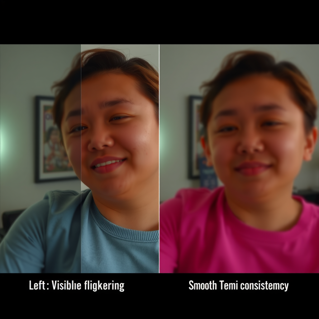
Flickering and High-Frequency Temporal Noise
Flickering manifests as rapid, frame-to-frame variations in pixel values or feature representations that create visual instability. This artifact typically originates from insufficient temporal regularization in the denoising process. The diffusion model's iterative refinement can introduce independent noise at each frame without adequate temporal constraints.
Mathematically, flickering can be quantified using temporal variance metrics. For a pixel location (x, y) across frames, the temporal variance is:
σ²_temporal(x,y) = (1/T) Σ[I_t(x,y) - μ(x,y)]²

Where:
I_t(x,y) = pixel intensity at frame t
μ(x,y) = temporal mean intensity
T = total number of frames
High temporal variance in regions that should remain static indicates flickering. Effective mitigation strategies include temporal smoothing losses, optical flow-guided consistency constraints, and multi-frame conditioning during the denoising process.
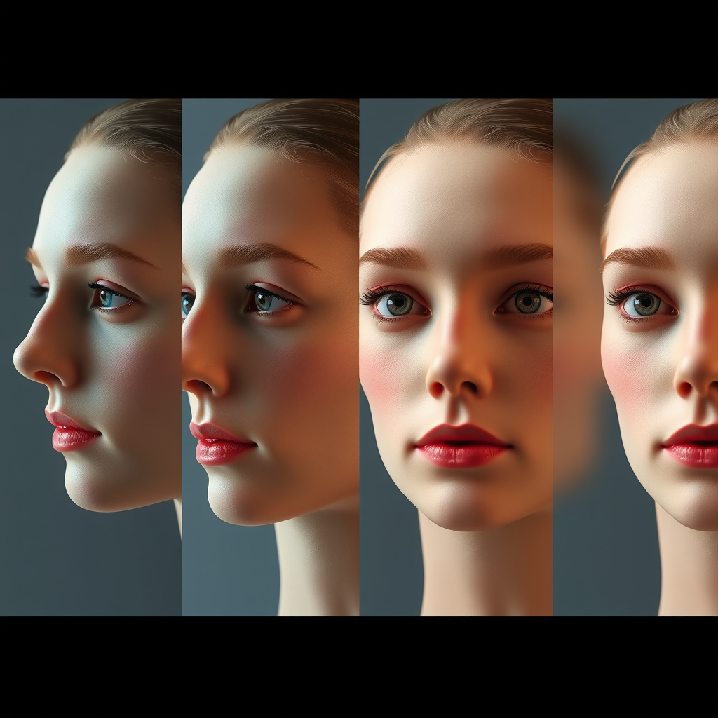
Morphing and Identity Drift
Morphing artifacts occur when object identities gradually change across frames, causing faces to shift features, objects to transform shapes, or textures to evolve unnaturally. This phenomenon reflects insufficient long-range temporal dependencies in the model architecture.
Identity drift can be measured using perceptual similarity metrics across temporal windows. The LPIPS (Learned Perceptual Image Patch Similarity) distance between frames provides a robust measure:
LPIPS(I_t, I_{t+k}) = Σ_l w_l · ||φ_l(I_t) - φ_l(I_{t+k})||²

Where:
φ_l = features from layer l of pretrained network
w_l = layer-specific weights
k = temporal offset
Excessive LPIPS distance growth with increasing temporal offset indicates identity drift. Mitigation approaches include reference frame conditioning, where early frames serve as anchors for identity preservation, and explicit identity embedding that remains constant across the sequence.
Research-Backed Strategies for Improving Temporal Coherence
Recent academic research has identified several effective strategies for enhancing temporal coherence in video generation models. These approaches combine architectural innovations, training methodologies, and inference-time techniques.
Latent Space Temporal Smoothing
Operating in latent space rather than pixel space provides computational advantages and enables more effective temporal regularization. The latent diffusion framework naturally supports temporal smoothing through latent-space constraints.
A temporal smoothness loss can be applied in latent space:
L_temporal = Σ_t ||z_t - z_{t-1}||² + α · ||∇_t z_t||²

Where:
z_t = latent representation at frame t
∇_t z_t = temporal gradient of latent
α = regularization strength
This loss encourages smooth transitions in latent space while the gradient term penalizes rapid temporal changes. Empirical results from recent papers show that α values between 0.1 and 0.5 effectively reduce flickering without over-smoothing motion.
Optical Flow-Guided Consistency
Optical flow provides explicit motion information that can guide temporal consistency. By computing flow fields between adjacent frames, the model can enforce that pixel movements follow physically plausible trajectories.
The flow-guided consistency loss warps previous frames according to estimated flow and penalizes deviations:
L_flow = Σ_t ||I_t - W(I_{t-1}, F_{t-1→t})||²

Where:
W(I, F) = warping operation using flow F
F_{t-1→t} = optical flow from frame t-1 to t
I_t = generated frame at time t
This approach has shown particular effectiveness in preserving object boundaries and maintaining texture consistency during motion. However, it requires accurate flow estimation, which can be challenging in regions with occlusions or complex deformations.
Multi-Frame Conditioning and Context Windows
Rather than generating frames independently or with only single-frame conditioning, multi-frame approaches condition each frame on multiple previous frames. This provides richer temporal context and enables the model to learn longer-range dependencies.
The conditioning mechanism concatenates features from multiple frames:
c_t = Concat[E(I_{t-k}), E(I_{t-k+1}), ..., E(I_{t-1})]

Where:
E(·) = encoder network
k = context window size
c_t = conditioning vector for frame t
Experiments with context windows of 4-8 frames show significant improvements in temporal coherence metrics. The trade-off involves increased memory requirements and computational cost, which can be mitigated through efficient attention mechanisms and gradient checkpointing.
Implementation Examples and Code Patterns
Practical implementation of temporal coherence mechanisms requires careful attention to computational efficiency and numerical stability. Below are code patterns demonstrating key concepts.
Temporal Attention Layer Implementation
import torch
import torch.nn as nn

class TemporalAttention(nn.Module):
    def __init__(self, dim, num_heads=8, window_size=5):
        super().__init__()
        self.num_heads = num_heads
        self.window_size = window_size
        self.scale = (dim // num_heads) ** -0.5

        self.qkv = nn.Linear(dim, dim * 3)
        self.proj = nn.Linear(dim, dim)

    def forward(self, x):
        # x shape: (batch, time, height, width, channels)
        B, T, H, W, C = x.shape

        # Reshape for attention computation
        x_flat = x.view(B, T, H*W, C)
        qkv = self.qkv(x_flat).reshape(B, T, H*W, 3,
                                        self.num_heads,
                                        C // self.num_heads)
        qkv = qkv.permute(3, 0, 4, 1, 2, 5)
        q, k, v = qkv[0], qkv[1], qkv[2]

        # Compute temporal attention within window
        attn_output = []
        for t in range(T):
            t_start = max(0, t - self.window_size // 2)
            t_end = min(T, t + self.window_size // 2 + 1)

            q_t = q[:, :, t:t+1]  # Current frame query
            k_window = k[:, :, t_start:t_end]  # Keys from window
            v_window = v[:, :, t_start:t_end]  # Values from window

            attn = (q_t @ k_window.transpose(-2, -1)) * self.scale
            attn = attn.softmax(dim=-1)

            out = (attn @ v_window).squeeze(2)
            attn_output.append(out)

        attn_output = torch.stack(attn_output, dim=2)
        attn_output = attn_output.transpose(1, 2).reshape(B, T, H*W, C)

        output = self.proj(attn_output)
        return output.view(B, T, H, W, C)
This implementation demonstrates a sliding window temporal attention mechanism that balances computational efficiency with temporal modeling capacity. The window size parameter controls the temporal receptive field.
Temporal Smoothness Loss
def temporal_smoothness_loss(latents, alpha=0.3):
    """
    Compute temporal smoothness loss in latent space

    Args:
        latents: Tensor of shape (batch, time, channels, height, width)
        alpha: Weight for gradient penalty term

    Returns:
        Scalar loss value
    """
    # First-order temporal difference
    temporal_diff = latents[:, 1:] - latents[:, :-1]
    l1_loss = torch.mean(torch.abs(temporal_diff))

    # Second-order temporal gradient (acceleration)
    if latents.shape[1] > 2:
        temporal_grad = temporal_diff[:, 1:] - temporal_diff[:, :-1]
        gradient_penalty = torch.mean(torch.abs(temporal_grad))
    else:
        gradient_penalty = 0.0

    total_loss = l1_loss + alpha * gradient_penalty
    return total_loss


# Usage in training loop
def training_step(model, batch_frames, optimizer):
    optimizer.zero_grad()

    # Encode frames to latent space
    latents = model.encode(batch_frames)

    # Standard reconstruction loss
    reconstructed = model.decode(latents)
    recon_loss = F.mse_loss(reconstructed, batch_frames)

    # Add temporal smoothness constraint
    smooth_loss = temporal_smoothness_loss(latents, alpha=0.3)

    # Combined loss
    total_loss = recon_loss + 0.1 * smooth_loss

    total_loss.backward()
    optimizer.step()

    return total_loss.item()
The temporal smoothness loss can be integrated into existing training pipelines with minimal modifications. The alpha parameter should be tuned based on the desired trade-off between temporal stability and motion preservation.
Quantitative Evaluation Metrics
Rigorous evaluation of temporal coherence requires metrics that capture both perceptual quality and objective consistency. Recent research has established several standard metrics for video generation assessment.
Temporal Consistency Score (TCS)
The Temporal Consistency Score measures frame-to-frame similarity using perceptual metrics. It aggregates LPIPS distances across all consecutive frame pairs:
TCS = 1 - (1/(T-1)) Σ_{t=1}^{T-1} LPIPS(I_t, I_{t+1})

Higher TCS indicates better temporal consistency
Typical range: 0.7 - 0.95 for good quality videos
TCS provides a single scalar that summarizes temporal stability. However, it should be complemented with motion-aware metrics that distinguish between legitimate motion and unwanted artifacts.
Warping Error Metric
The warping error quantifies how well frames align after optical flow compensation. This metric specifically targets motion-related inconsistencies:
WE = (1/(T-1)) Σ_{t=1}^{T-1} ||I_t - W(I_{t-1}, F_{t-1→t})||₁

Lower WE indicates better motion consistency
Normalized by image intensity range [0, 1]
Warping error is particularly sensitive to morphing artifacts and helps identify cases where object identities drift over time despite smooth frame transitions.
Frechet Video Distance (FVD)
FVD extends the Frechet Inception Distance to video by computing statistics over spatiotemporal features extracted from a pretrained 3D CNN. It measures the distributional similarity between generated and real videos:
FVD = ||μ_real - μ_gen||² + Tr(Σ_real + Σ_gen - 2√(Σ_real·Σ_gen))

Where:
μ_real, μ_gen = mean feature vectors
Σ_real, Σ_gen = covariance matrices
Lower FVD indicates better quality
FVD has become the standard metric for video generation benchmarks, though it requires large sample sizes for reliable estimation and can be sensitive to the choice of feature extractor network.
Future Directions and Open Challenges
Despite significant progress in temporal coherence mechanisms, several fundamental challenges remain open areas of active research. Addressing these challenges will be crucial for advancing video generation capabilities toward production-quality applications.
Long-Range Temporal Dependencies
Current architectures struggle with maintaining consistency over sequences longer than a few seconds. The quadratic complexity of attention mechanisms limits practical temporal window sizes, while hierarchical approaches introduce their own challenges in propagating information across temporal scales.
Promising research directions include sparse attention patterns that selectively attend to key frames, memory-augmented architectures that maintain explicit state across long sequences, and hybrid approaches combining attention with recurrent mechanisms for efficient long-range modeling.
Physics-Informed Temporal Constraints
Incorporating physical priors about motion, lighting, and object permanence could significantly improve temporal coherence. Current models learn these constraints implicitly from data, but explicit physics-based regularization might enable better generalization and more realistic dynamics.
Research in this direction explores differentiable physics simulators integrated into the generation pipeline, learned dynamics models that enforce physical plausibility, and hybrid approaches that combine data-driven generation with physics-based refinement.
Computational Efficiency
The computational cost of video generation with strong temporal coherence remains prohibitive for many applications. A single high-quality video sequence can require hours of GPU time, limiting iterative refinement and real-time applications.
Efficiency improvements are being pursued through model distillation, where smaller student models learn to approximate larger teacher models, progressive generation strategies that refine temporal resolution gradually, and architectural innovations like efficient attention mechanisms and conditional computation that activate only necessary components.
Conclusion
Temporal coherence represents one of the most critical challenges in modern video generation systems. While significant progress has been made through sophisticated attention mechanisms, temporal regularization techniques, and flow-guided consistency constraints, substantial room for improvement remains.
The mathematical frameworks presented in this article provide a foundation for understanding and addressing temporal artifacts. Temporal attention mechanisms enable models to capture dependencies across frames, while metrics like temporal consistency scores and warping error quantify the quality of generated sequences.
Practical implementation requires careful balancing of computational efficiency, temporal window sizes, and regularization strengths. The code examples demonstrate how these concepts translate into working systems, though optimal hyperparameters remain task-dependent and require empirical tuning.
Looking forward, the integration of physics-based priors, more efficient architectures for long-range dependencies, and improved training methodologies promise to push video generation capabilities closer to production-quality applications. As research continues to address these challenges, we can expect increasingly coherent and realistic video synthesis across diverse domains and use cases.
The field of video generation stands at an exciting juncture where theoretical understanding, architectural innovations, and computational capabilities are converging to enable new possibilities. Continued focus on temporal coherence mechanisms will be essential for realizing the full potential of these systems.